Support Vector Machine with Kernel

Step by step : Example from banking.csv data set.

What is SVM in terms of Machine Learning view point?

In machine learning there are two types of algorithms.

1. Unsupervised algorithms: Identify the patterns using untagged data.
2. Supervised algorithms: The data is tagged by the human. Identify the patterns or clusters using known data.

So, the SVM is a very powerful and flexible supervised machine learning algorithm.

Why SVM…?

Today with the growth of machine learning applications the Support vector machines are used in large amount of applications.

1. Handwriting recognition
2. Instruction detection
3. Face detection
4. Email classification
5. Gene classification

The major advantage why we using SVMs on above application is it can handle both “classification” and “regression” on both “linear” and “non-linear” data. It is the extended version of linear classifier and it usually gives a high accuracy.

Lets get in to the example | Using google collab notebook in python

There are few steps we have to follow before applying the SVM kernel functions to the dataset. Because we are getting a raw data set.

Steps to building a ML model

Procedure of building a machine learning model

first and foremost we have to upload the data set into our drive and create a blank collab notebook. You can get the data set using the bellow link.

Meet Google Drive - One place for all your files

First import the data to the drive and connect the drive to load the data.

#To give the access to the drive
from google.colab import drive
drive.mount("/content/gdrive")

Using pandas read_csv() can load the data. inside the brackets we have to give the path of the dataset.

#import data
import pandas as pd
df = pd.read_csv("/content/gdrive/My Drive/d/banking.csv")
df.head()

After loading the data we can view it using df.head(). inside the brackets we can give the number of columns we want to view. if not as default it is giving the first 5 raws as bellows.

Data frame

Import libraries

import pandas as pd
from sklearn import metrics
from sklearn.preprocessing import FunctionTransformer
import numpy as np
import seaborn as sns
from sklearn.preprocessing import StandardScaler,MinMaxScaler ,LabelEncoder
import matplotlib.pyplot as plt
import scipy.stats as stats
from sklearn.decomposition import PCA
import math
from sklearn.metrics import confusion_matrix

01. DATA CLEANCING

df.shape gives us number of rows and columns.

df.shape
output:(41188, 21)

df.info() gives the all information about the data set.

df.info()
df.describe(include=all)

Duplicate value check

check whether there are duplicate values. if available we have to remove. luckily our dataset has no duplicates

df.duplicated(subset=None, keep='first'

Check null values. we can get the sum of null values column wise using bellow code block.

df.isnull().sum()

Data set have both numerical and categorical data. Therefore it is easy to process further by dividing the dataset into categorical and numerical

#seperate data set
numeric_data = df.select_dtypes(include=[np.number])
categorical_data = df.select_dtypes(exclude=[np.number])

Outliers checking

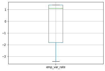
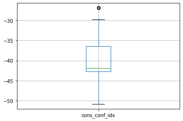
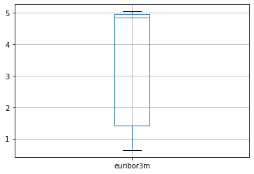
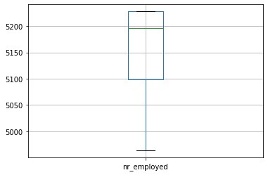
We can draw boxplot to see the outliers

numeric_data.boxplot()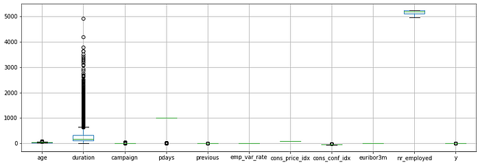

Boxplot for numerical data

In some cases we have to handle the outliers. But SVM kernel functions have least sensitivity for outliers. There are ways to handle outliers.

1. Drop the outliers

print('pdays 0 rows count', temp_df[temp_df[feature_name] <= 100].count())
df = df[df[feature_name] >= 100]
print(df.shape)

1. Handle the outliers using IQR method.

#Handling outliers of age
fig, axes = plt.subplots(1,2)
plt.tight_layout(0.2)
print("Previous Shape With Outlier: ",df.shape)
sns.boxplot(df['age'],orient='v',ax=axes[0])
axes[0].title.set_text("Before")
Q1 = df["age"].quantile(0.25)
Q3 = df["age"].quantile(0.75)
print(Q1,Q3)
IQR = Q3-Q1
print(IQR)
lower_limit = Q1 - 1.5*IQR
upper_limit = Q3 + 1.5*IQR
print(lower_limit,upper_limit)
df3 = df
df3['age'] = np.where(df3['age']>upper_limit,upper_limit,df3['age'])
df3['age'] = np.where(df3['age']<lower_limit,lower_limit,df3['age'])
print("Shape After Removing Outliers:", df3.shape)
sns.boxplot(df3['age'],orient='v',ax=axes[1])
axes[1].title.set_text("After")
plt.show()
df['age'] = df3['age']

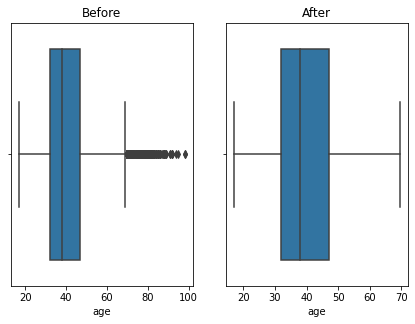
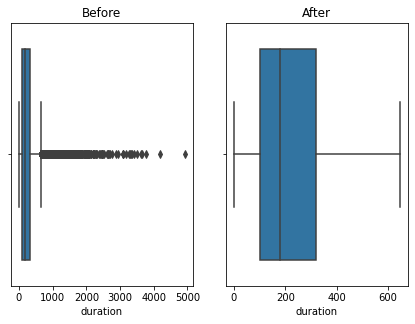
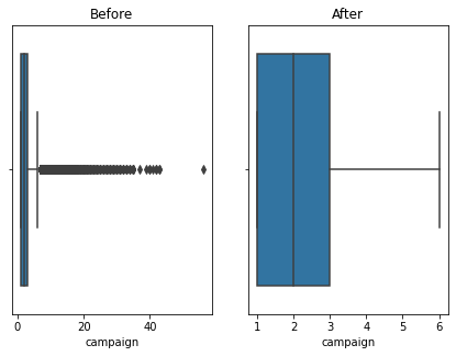
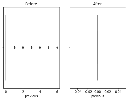
Here using the banking dataset we got some outliers. After handling the outliers we loose some data. Actually this is also class imbalanced data so data loss will affect for the accuracy. I tried the accuracy before handling the outliers and after handling the outliers. So i got a better accuracy without handling outliers. Also some says that tree based algorithms are not sensitivity to the outliers. So practically with the data set we got a better accuracy without handling outliers.

2. Data Transformations

Any data scientist prefer if data comes from Normal Distribution. But the real scenario is the data comes from the real data set will follow more skewed distributions. we use transformation techniques to map skewed distribution to normal distribution.

By visualizing the data as histograms we can get weather the distribution is a normal or skewed, if skewed whether it is right skewed or left skewed. According to the skewness we apply different transformation techniques

numeric_data.hist(figsize=(10,10))

Hostograms before transform

#Do the  trasnformations for required features
sqrt_transformer = FunctionTransformer(np.sqrt) # For Left Skewed Data
exp_transformer = FunctionTransformer(np.exp) # For Right Skewed Data
lambda_transformer = FunctionTransformer(lambda x: x**2, validate=True ) # For Right Skewed Data
# load your data
# apply the transformation to data
data_age = sqrt_transformer.transform(df['age'])
data_duration =  sqrt_transformer.transform(df['duration'])
data_campaign = sqrt_transformer.transform(df['campaign'])
#data_emp_var_rate = sqrt_transformer.transform(df['emp_var_rate'])
#data_previous = sqrt_transformer.transform(df['previous'])
#data_euribor3m =  exp_transformer.transform(df['euribor3m'])
#data_nr_employed = lambda_transformer.transform(df['nr_employed'])
#data_cons_conf_idx = reciprocal_transformer.transform(df['cons_conf_idx'])
numeric_data['age']=data_age
numeric_data['duration']=data_duration
numeric_data['campaign']=data_campaign
#numeric_data['previous']=data_previous
#numeric_data['emp_var_rate']=data_emp_var_rate
#numeric_data['euribor3m']=data_euribor3m
#numeric_data['nr_employed']=data_nr_employed
#numeric_data['cons_conf_idx']=data_cons_conf_idx
#plot the histrogram again to see how transformation affected
numeric_data.hist(figsize=(10,10))

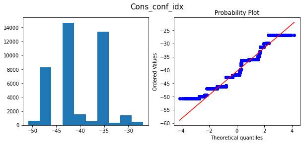
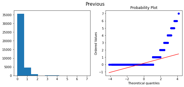
only applying the transformation for the features “age”,”compaign”, “duration” we can get high accuracy

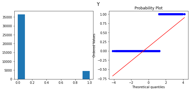
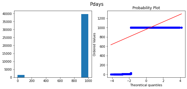
Histograms and Q-Q plots after transform

3. Feature Coding

We are dealing with numeric data. but real data has categorical data. Since the machine learning algorithms works only for numerical data we need to encode them. One hot encoding and label encoding are two ways of encoding. while the one hot encoding is the best. Because it only consider the 0 and 1. If the features got values 0,1,2,3,4… like this the algorithm may confuse 0 has the low value and 4 has the highest value. since we are using banking data set and SVM kernel fumcton for prediction we can use lable encoding. because this algorithm perform equally for both.

# Use label encorder
labelencoder = LabelEncoder()
df['job']= labelencoder.fit_transform(categorical_data['job'])
df['marital']= labelencoder.fit_transform(categorical_data['marital'])
df['education']= labelencoder.fit_transform(categorical_data['education'])
df['default']= labelencoder.fit_transform(categorical_data['default'])
df['housing']= labelencoder.fit_transform(categorical_data['housing'])
df['loan']= labelencoder.fit_transform(categorical_data['loan'])
df['contact']= labelencoder.fit_transform(categorical_data['contact'])
df['month']= labelencoder.fit_transform(categorical_data['month'])
df['day_of_week']= labelencoder.fit_transform(categorical_data['day_of_week'])
df['poutcome']= labelencoder.fit_transform(categorical_data['poutcome'])
print(df.info())
df.head(5)

Relation between each features

sns.pairplot(df, hue='y', vars=['age', 'duration', 'campaign', 'pdays', 'previous',
       'emp_var_rate', 'cons_conf_idx', 'job', 'marital',
       'default', 'housing', 'month', 'day_of_week',
       'poutcome'])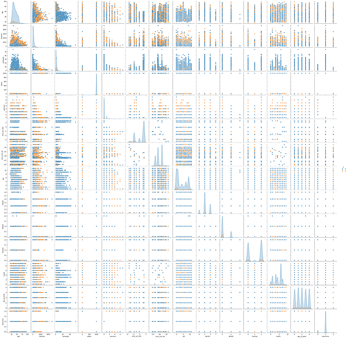

4.Feature Scaling

The data set there are different units values from different ranges. So it is easy if we can scale down the values. Therefore using feature scalling techniques we can scale down the values.

#remove target variable 
independent=numeric_data.drop(columns=["y"])

we use MinMaxScaler and StandradScaller. We need to use only one. why i mention both is here i got good acuracy from StandradScaller rather then the MinMaxScaler.

# Getting Column Names
cat_columns=categorical_data.columns
columns_values = independent.columns
target = numeric_data['y'] 
#Applying Standardization 
#step 1 - Calling the standard scaler
#scaler = StandardScaler()
scaler = MinMaxScaler()
scaler.fit(independent) 
X_Scaled = scaler.transform(independent)
X_Scaled_df =  pd.DataFrame(X_Scaled,columns=columns_values)
X_Scaled_Except = pd.DataFrame(df,columns=cat_columns)
X_standard = X_Scaled_df.join(X_Scaled_Except)
X_standard = X_standard.join(target)
#X_standard= pd.DataFrame(X_standard,numeric_data['y'] )
X_standard.info()
X_standard

5. Feature Extraction

By now we have 21 features. If we use one hot encoding we are getting lot more features. Actually since this is real data all the features may not be needed to the final prediction. But the thing is we don’t know which are needed and which are not needed. Therefore to reduce the large no of features we can use feature reduction.

#Heat map to find relatonship between each feature
X_standard.corr()
#Heat map to find relatonship between each feature
fig_dims = (15, 10)
fig, ax = plt.subplots(figsize=fig_dims)
sns.heatmap(X_standard.corr(),ax=ax)

Correlation matrix

See we can identify there are featues correlaed. We can keep one and drop the others. To get a better confirmation we can use diferent values and check our model acuracy. Bellow code fragment helps you to find the corelated feature pairs.

#finding co related features
def correl(X_standard):
    cor = X_standard.corr()
    corrm = np.corrcoef(X_standard.transpose())
    corr = corrm - np.diagflat(corrm.diagonal())
    print("max corr:",corr.max(), ", min corr: ", corr.min())
    c1 = cor.stack().sort_values(ascending=False).drop_duplicates()
    high_cor = c1[c1.values!=1]
    ## change this value to get more correlation results        
    thresh = 0.7
    display(high_cor[high_cor>thresh])
correl(X_standard)
Output:
max corr: 0.9722446711516148 , min corr:  -0.5875138561368151
euribor3m     emp_var_rate      0.972245
nr_employed   euribor3m         0.945154
              emp_var_rate      0.906970
emp_var_rate  cons_price_idx    0.775334
dtype: float64
#drop corelated columns
X_standard=X_standard.drop(columns=["emp_var_rate","nr_employed"])

Proncipal Component Analycis

#removing target 
X=X_standard.drop(columns=["y"])
X=X_standard.dropna()
#removing target 
X=X_standard.drop(columns=["y"])
X=X_standard.dropna()
print(X_pca.shape)
X_before_pca = X
X=X_pca

Data Generation and Class Imbalance

Class imbalance is a one of problem with the dataset. Simply we can say that the target class “y” s frequency is highly imbalanced. We can observe that plotting a graph like this.

#checking class imbalance
y_true = X_standard['y']
print(X_standard['y'].value_counts())
sns.countplot(x='y', data=X_standard)
plt.show()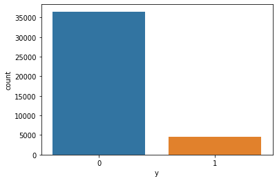

y class imbalance

So it can be identify most of the y values are 0 and compared to them 1 values are very less. In order to train the model properly and getting high accuracy we have to balance the train data class values.

from imblearn.over_sampling import SMOTE
from sklearn.model_selection import train_test_split
os = SMOTE(random_state=0)
X.shape
X_class_train, x_test, y_class_train, y_test = train_test_split(X, y_true, test_size=0.2, random_state=0)
data_X, data_y = os.fit_sample(X_class_train, y_class_train)
smoted_X = pd.DataFrame(data=data_X )
smoted_y= pd.DataFrame(data=data_y,columns=['y'])
sns.countplot(x='y', data=smoted_y)
plt.show()

After removing class imbalance

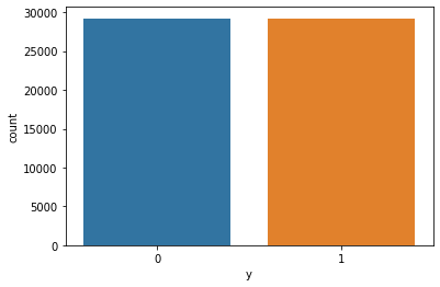
So now the class is balanced.

9. Apply the smoted data to Train dataset

Above we apply smote technique to remove the calss imbalance. So Now it should assign to the train set.

x_train = smoted_X
y_train = smoted_y
y_train=y_train.values.ravel()
print("Traing Data Shape",x_train.shape, y_train.shape)
print("Testing Data Shape",x_test.shape, y_test.shape)
Output:
Traing Data Shape (58446, 10) (58446,)
Testing Data Shape (8238, 10) (8238,)

10. Modeling SVM with Kernel functions.

There are five different kernel functions.

1. Linear
2. Poly
3. RBF
4. Gaussian
5. Sigmoid

In this example I did not apply gaussian kernel. But all the other kernel functions i have tried showing bellow with the accuracy.

First of all we need to include below libraries.

#import libraries  for svm 
from sklearn.svm import SVC
from sklearn.calibration import CalibratedClassifierCV
from sklearn.metrics import roc_auc_score
from sklearn.metrics import classification_report, confusion_matrix

1. Support Vector Machines with Linear Kernel function

SVC() method we can pass so many parameters. Here i used 3 of them.

• kernel − string, optional, default = ‘rbf’

This parameter specifies the type of kernel to be used in the algorithm. we can choose any one among, ‘linear’, ‘poly’, ‘rbf’, ‘sigmoid’, ‘precomputed’. The default value of kernel would be ‘rbf’.

• gamma − {‘scale’, ‘auto’} or float,

It is the kernel coefficient for kernels ‘rbf’, ‘poly’ and ‘sigmoid’.

• C − float, optional, default = 1.0

It is the penalty parameter of the error term.

from sklearn import svm
classifier=svm.SVC(kernel='linear', gamma='auto', C=2)
classifier.fit(x_train,y_train)
y_predict_linear=classifier.predict(x_test)

After getting few times the model is trained. and now using the model we can predict the y values. Below graph shows the performance of the model.

class_names = ['negative','positive']
df_heatmap = pd.DataFrame(confusion_matrix(y_test, y_predict_linear), index=class_names, columns=class_names)
fig = plt.figure( )
heatmap = sns.heatmap(df_heatmap, annot=True, fmt="d")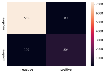

print(classification_report(y_test, y_predict_linear))
output:
              precision    recall  f1-score   support
           0       0.99      0.99      0.99      7325
           1       0.90      0.88      0.89       913
accuracy                           0.98      8238
   macro avg       0.94      0.93      0.94      8238
weighted avg       0.98      0.98      0.98      8238

2. Support Vector Machines with Poly Kernel function

from sklearn import svm
classifier=svm.SVC(kernel='poly', gamma='auto', C=2)
classifier.fit(x_train,y_train)
y_predict_poly=classifier.predict(x_test)
class_names = ['negative','positive']
df_heatmap = pd.DataFrame(confusion_matrix(y_test, y_predict_poly), index=class_names, columns=class_names)
fig = plt.figure( )
heatmap = sns.heatmap(df_heatmap, annot=True, fmt="d")

print(classification_report(y_test, y_predict_poly))
Output:
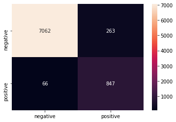
              precision    recall  f1-score   support
           0       0.99      0.96      0.98      7325
           1       0.76      0.93      0.84       913
accuracy                           0.96          8238
   macro avg       0.88      0.95      0.91      8238
weighted avg       0.97      0.96      0.96      8238

3. Support Vector Machines with RBF Kernel function

model =SVC(kernel="rbf" ,C = 2)
clf = CalibratedClassifierCV(model, cv=3)
clf.fit(x_train,y_train)
model.fit(x_train,y_train)
y_predict_rbf=model.predict(x_test)
pred_test = clf.predict_proba(x_test)[:,1]
fpr1, tpr1, thresholds1 = metrics.roc_curve(y_test, pred_test)
pred_train = clf.predict_proba(x_train)[:,1]
fpr2,tpr2,thresholds2 = metrics.roc_curve(y_train,pred_train)

cnxxc

print("AUC on Test data is " +str(roc_auc_score(y_test,pred_test)))
print("AUC on Train data is " +str(roc_auc_score(y_train,pred_train)))
Output:

AUC on Test data is 0.9639143355924474
AUC on Train data is 0.9745059334731189

ass

class_names = ['negative','positive']
df_heatmap = pd.DataFrame(confusion_matrix(y_test, y_predict_rbf), index=class_names, columns=class_names)
fig = plt.figure( )
heatmap = sns.heatmap(df_heatmap, annot=True, fmt="d")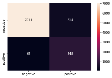

print(classification_report(y_test, y_predict_rbf))
output: 
              precision    recall  f1-score   support
           0       0.99      0.96      0.97      7325
           1       0.73      0.93      0.82       913
accuracy                           0.95      8238
   macro avg       0.86      0.94      0.90      8238
weighted avg       0.96      0.95      0.96      8238

After all we can see the best accuracy is getting from the SVM linear model.